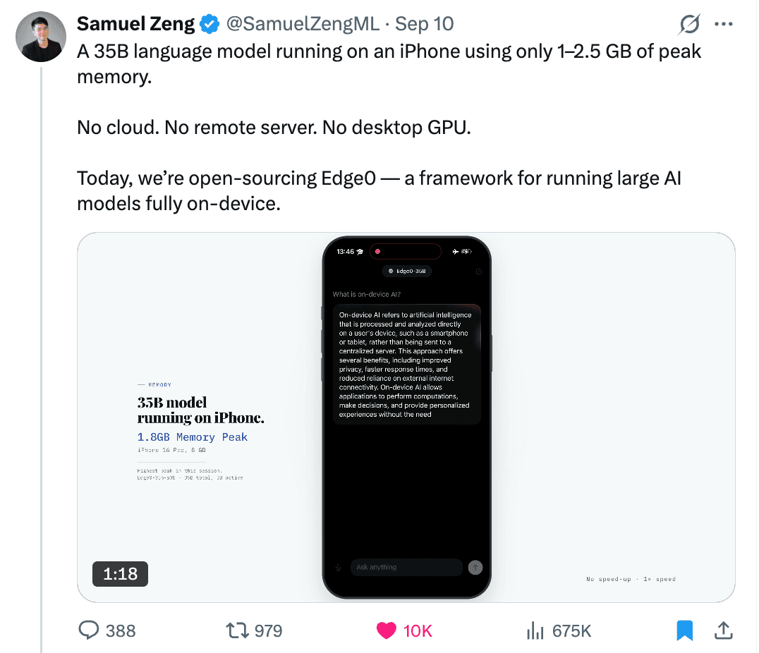
On September 10, we officially open-sourced Edge0 — a major breakthrough for on-device AI.
For the first time, on consumer hardware — phones, PCs, smart devices and embodied robots — we ran large-parameter models “with extremely low memory,” breaking through the “memory wall” that has long constrained on-device AI.
Put simply, Edge0 lets a 35-billion-parameter language model run on an ordinary phone with low power and low memory, at roughly 1–2.5 GB of peak active memory. In other words, a phone can run a large-parameter model with about the same resource footprint as scrolling short videos.
Edge0 targets phones, computers, robots and other devices, and is suited to building local AI applications that run offline with low power and a small memory footprint.
In the first week after the release, Edge0 drew significant attention from overseas communities. Posts by founder Dr. Xiaodong Zeng on X and LinkedIn accumulated over 1 million views, and the model reached Top 1 on Hugging Face’s overall model trending list. Meanwhile, developers have already begun building on Edge0’s models and framework, exploring more on-device scenarios.
In this article, we want to share why we built Edge0, and how we thought about on-device large models throughout the R&D process.
Before We Begin
Over the past four years, the fiercest battle in large-model research has not been fought on leaderboards, but in memory.
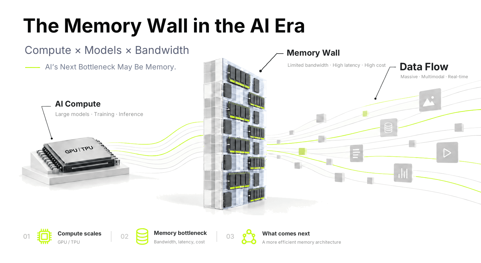
“Memory wall” is not a term of the AI era. In 1995, computer-architecture researchers Wulf and McKee wrote a paper titled “Hitting the Memory Wall.” Their concern was simple: processors get faster every year, while memory barely keeps up. What holds a system back is often not how slowly it computes, but how slowly it moves data.
Thirty years on, the same wall has risen again in a new place — this time in front of AI.
Over the past four years, the industry’s hottest topic has been compute: how many cards, how many trillions of floating-point operations, how many billions of dollars. But what actually decides whether a model can run, how fast it runs, and who can afford it is often memory: where to put tens of gigabytes of weights, where to put the cache that grows with the conversation, how many bytes must be moved for each generated token. This article is about the shape of that wall in the AI era, and how far we have gotten.
1. The Bottleneck Is Not Compute, It’s Memory
A 35-billion-parameter model, after 4-bit quantization, needs more than 20 GB for weights alone; add the conversation context and intermediate results, and an ordinary computer’s memory cannot hold it. This is the most intuitive explanation — and the one most easily mistaken for the whole story.
The industry long ago offered a more precise explanation: the bottleneck is memory.
Why not compute? Because in the generation phase, for every token the model emits, it must move “all weights + the entire context” across the memory bus once, and the floating-point work done during that trip is pitifully small. In other words, the price tag of this step is bytes, not operations. No amount of compute can route around the movement.
How bad is the waste? A 70-billion-parameter model (BF16) doing single-user decoding on an H100 spends 99.8% of its compute units’ time waiting for weights to arrive from HBM, reaching only 0.2% of the chip’s peak. To tell whether a workload is compute-bound or bandwidth-bound, look at arithmetic intensity: decoding does roughly one operation per byte moved, while this card’s balance point is around 295. Two orders of magnitude apart. Adding compute does not help; adding bandwidth does.
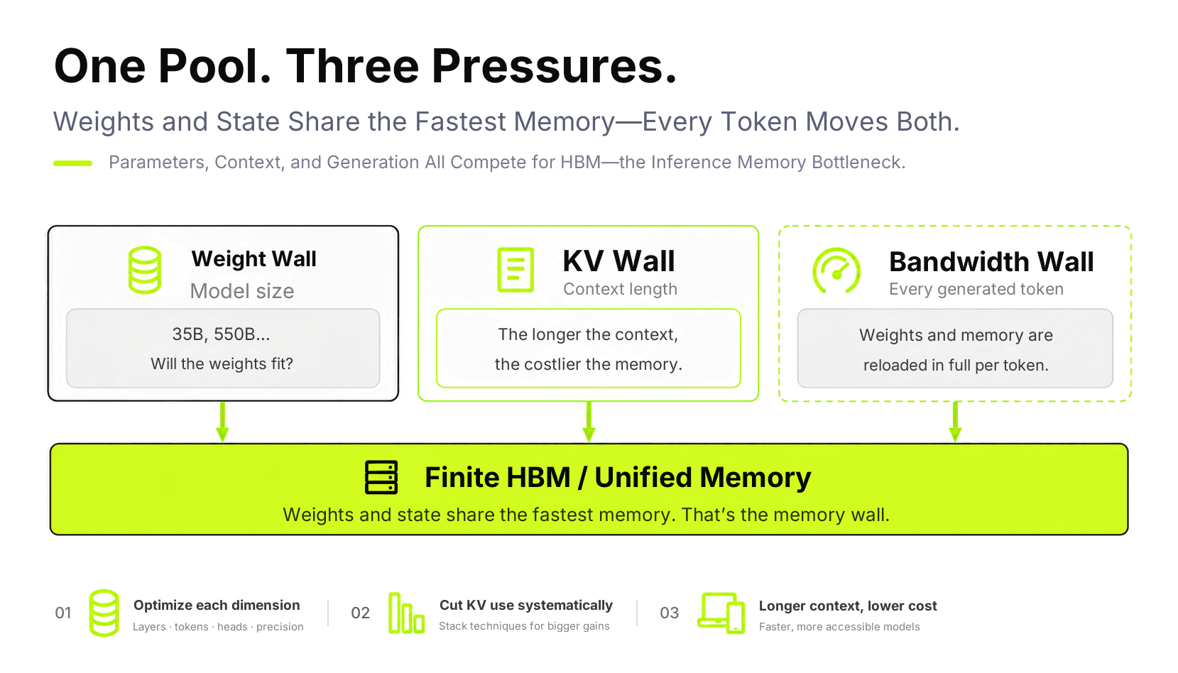
And under the word “memory” live two occupants with very different temperaments.
Weights are a static giant: tens of gigabytes, fixed after training, yet read in full for every generated token. State (the KV cache) is a dynamic grower: tiny at first, expanding linearly as the conversation lengthens, storing one more copy per additional token.
Their ways out differ: one side’s size is fixed from the start, the other keeps growing with the conversation. Over the past four years, the vast majority of public work in the industry went to the latter half; the real battlefield on-device is the former. We discuss them separately below.
2. The Weight Side: Shrink First, Then Hit the Wall
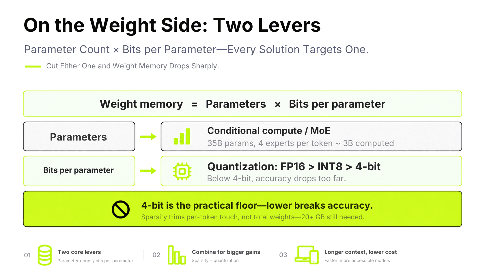
Weights have only one formula: parameter count × bits per parameter. Every method on the weight side lands on these two variables.
The precision axis is the most direct. Going from 16-bit to 8-bit is nearly lossless; 4-bit is today’s engineering sweet spot for on-device: 35 billion parameters therefore need only a bit over 20 GB.
Below that there is no road: beyond 4 bits, the error is too large to use. 2-bit and 1-bit still have no usable solution today. What drops is not one or two points but general capability collapsing across the board. The precision axis ends at 4 bits.
Even compressed to 4 bits, the weights of 35 billion parameters are still over 20 GB — they do not fit in an ordinary computer’s memory.
There is also an easily overlooked fact: these 35 billion parameters are not all on the field every time. The MoE structure means each token activates only 4 experts — about 3 billion parameters participate in computation; the rest are idle at that moment.
But “idle” does not mean “absent.” Those 20-plus GB must live somewhere, and an ordinary device’s memory is only so large: the data-center answer is more memory and more cards; on-device has no such road. That is the on-device wall itself.
3. The State Side: Why Longer Conversations Cost More
State is the opposite of weights. Weights are loaded once and reused; the KV cache appends one copy per generated token, and as long as the conversation continues it cannot be discarded. The next computation must read the history again — the longer the chat, the longer the read, the more expensive the bill.
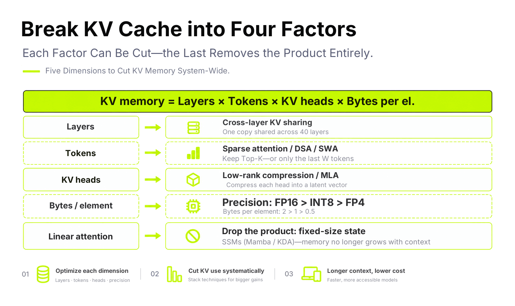
How much memory one KV cache occupies can be written as a multiplication: layers × tokens × KV head dimension × bytes per element. Four multipliers, each cuttable on its own.
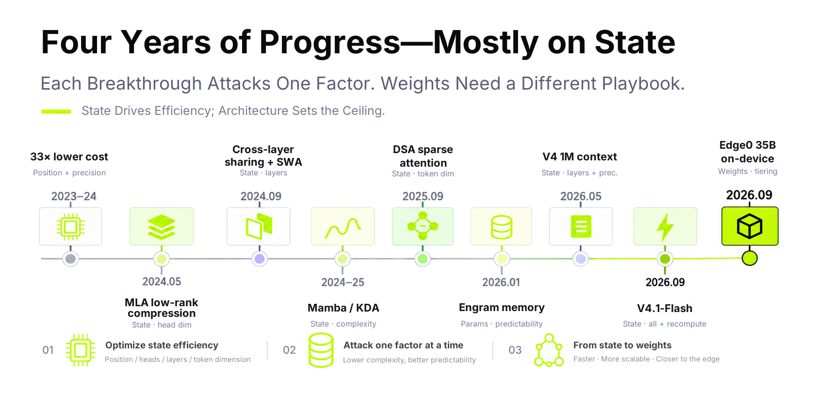
Each of the four routes has representative work; line them up in time:
A few worth calling out.
MLA (May 2024) compresses the old “one cache per head” into a low-rank vector. The official figure is a 93.3% reduction in KV cache relative to standard multi-head attention; it later became the foundation of the entire DeepSeek series, with all later sparsity stacked on top of it.
DSA (September 2025) takes another approach: instead of compressing the cache, it decides what to look at. A lightweight indexer first selects the ~2048 most relevant positions; the core attention’s complexity drops from O(L²) to O(Lk), and the official API price was cut by more than half soon after. The cost is written into the training pipeline: warm up with dense attention so the indexer learns to imitate the original distribution, then switch to sparse training.
Cross-layer sharing is the most direct move today: the caches of 40 layers are highly similar — why store 40 copies? By this September’s V4.1-Flash, it has been refined into assigning different patterns per layer — a few layers faithfully read the full context and produce a complete cache, while the rest directly reuse results computed by others.
There is an even more radical route: drop KV entirely. Work such as Mamba, DeltaNet and KDA replaces the length-growing state with a fixed-size vector, so memory no longer grows with context.
These routes look unrelated. But from another angle, they answer the same question: how should this cache be addressed.
Full attention is content addressing: match the current query against history item by item. Most precise, and the cost keeps rising with length.
Linear attention compresses history into a fixed-capacity state, equivalent to a lossy summary: constant capacity, details lost.
Sparse attention is two-step addressing: cheap coarse filtering first, then precise lookup.
Engram returns to the oldest scheme — hash addressing, O(1) table lookup; MoE decides which part of the parameters to use per token, equivalent to addressing over parameters.
Placed in one framework, the main line is clear: what the industry keeps changing is the addressing scheme; the goal never changes — preserve more precise recall with fewer bytes. Precisely because this bottom line exists, hybrid architectures became consensus: keeping 5% to 15% of expensive but precise layers is paying separately for “precision.”
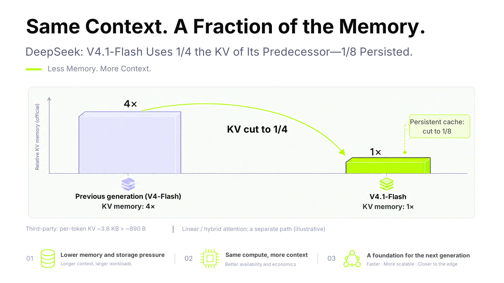
The effect is measurable. By DeepSeek’s official numbers, at 1M-token context V4 needs only 27% of V3.2’s per-token inference compute and 10% of its KV cache; with V4.1-Flash, KV occupancy drops again to 1/4 of the previous generation, and the persisted on-disk cache to 1/8.
A million-token context once meant unaffordable cost. Now it is becoming an engineering problem.
Looking back at the most-cited work of these four years together, nearly all of it cuts on the state side: MLA, sparse attention, sliding windows, linear attention — all point at KV. So much so that “memory optimization” is often equated with “KV optimization.” But the other half of the memory wall — those tens of gigabytes of weights — has never shrunk because KV shrank. On-device, it is what truly does not fit.
4. Where the Two Sides Meet: Spreading Across the Whole Storage Chain
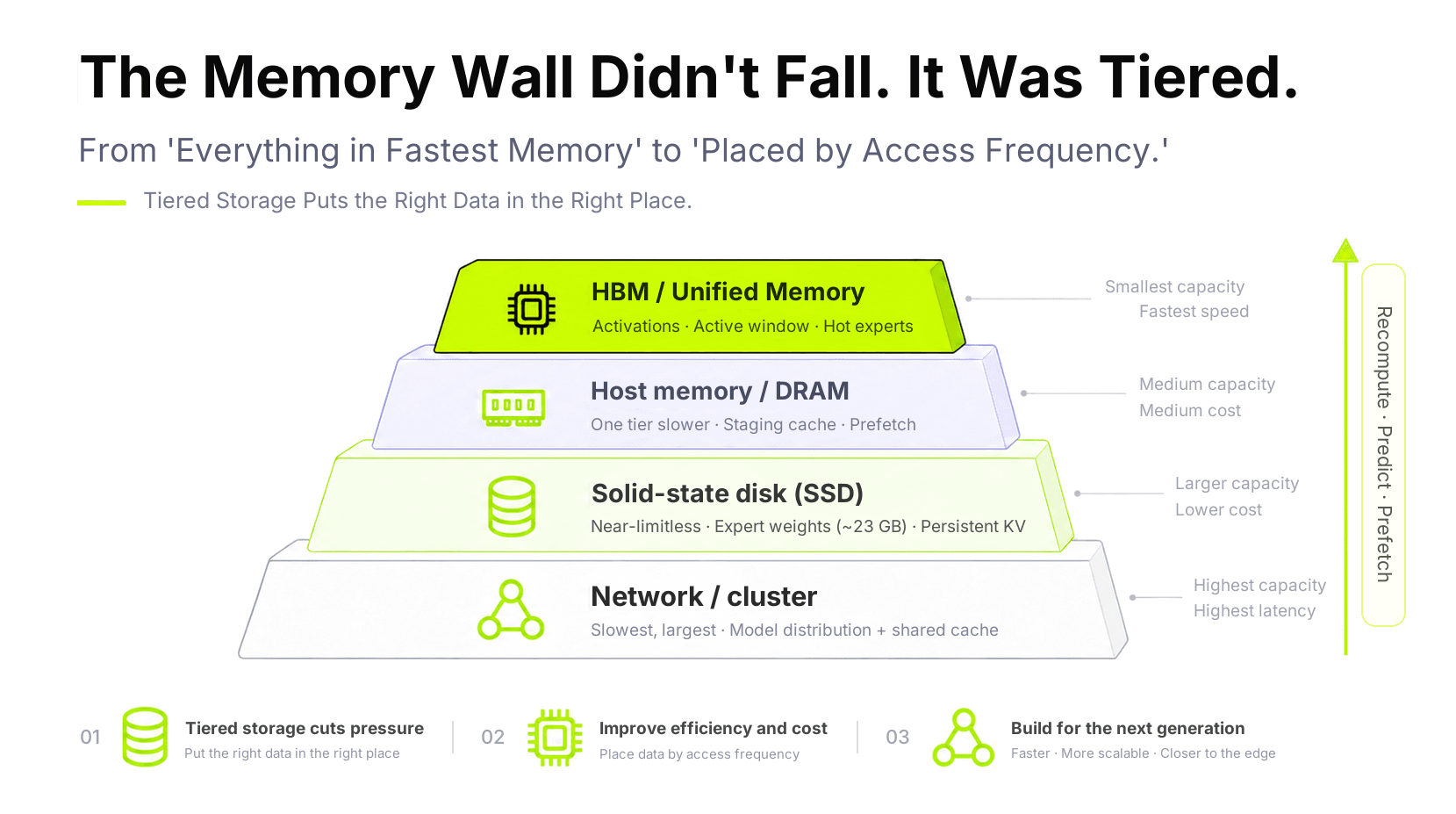
If compression is “making things smaller,” there is another half of the story: moving things elsewhere. On this step, weights and state are fellow travelers.
Keep only what is being computed in the fastest storage. Prefix caches, KV reused across turns, and static lookup data go to host memory. Weights go to SSD. Model distribution and shared caches go to the network.
The most notable entry on this line is Engram (January 2026). It modernizes classic N-gram table lookup, letting the model “look up” rather than “compute” part of its knowledge, placing a 100-billion-parameter memory table in host memory with less than 3% throughput loss.
What makes this possible? Because the table’s addresses are computable, so they can be fetched ahead. Hidden here is the precondition of the whole route: whether tiering works depends on whether access is predictable.
And this leads to the most counter-intuitive turn of this generation of architectures. In the past, “whether access is predictable” was a property of the workload itself — chats have sessions, documents have prefixes; hitting it was luck. Now it becomes a capability the model can design for itself: indexers are trainable, hashes are deterministic, routing is regular.
In other words, models are not just getting smaller and faster — they are starting to make way for the storage system. This is the change most worth remembering on this route: predictability goes from a kind of luck to a trainable capability.
5. On-Device: Squeezing Both Sides to the Limit
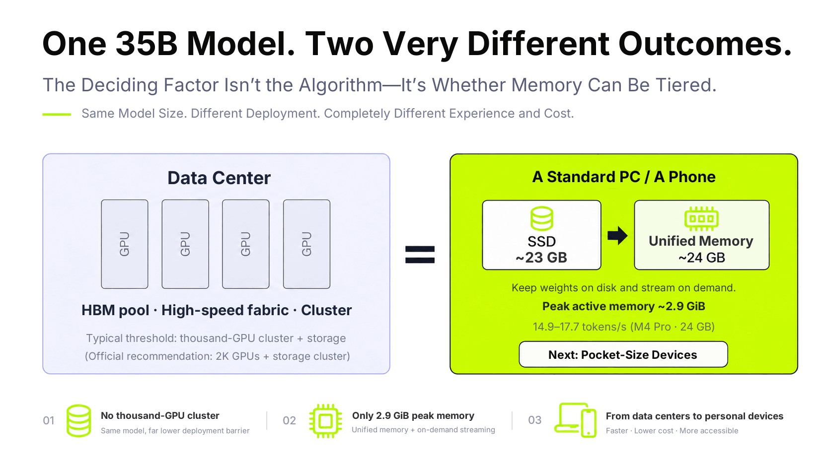
All the tiering above has an escape route in the data center: not enough bandwidth, add cards; not enough memory, add clusters. DeepSeek’s V4.1 release notes also state that large-scale deployment requires clusters and storage clusters at the 2000-card level.
On-device has none of these escapes. A 24 GB computer, or a phone, has only the memory and storage inside the machine: no high-speed interconnect, no scalable storage pool, not even a second machine.
To run a 35-billion-parameter model on such a device, one must accept two very awkward things at once.
First, accept this: at the edge, tiering means weights are not in memory most of the time. Our approach puts the full 4-bit weights on disk (~23 GB), streams them in on demand, and presses peak active memory down to the 2.9 GiB range, with decoding at 14.9 to 17.7 tokens/s (a Mac mini, M4 Pro, 24 GB unified memory).
Second, no waiting. Reading weights from disk has latency, and the wait happens exactly on the critical path of generating every token. Once you start waiting, speed is gone.
The state side is equally unavoidable. The 2.9 GiB above is a short-context number; as context grows, so does it: with a 3.3k-token input, the 8b tier’s peak active memory reaches about 3.3 GiB, and the increase is mostly KV. Both sides must be saved — that is exactly why on-device is harder than the data center.
And “no waiting” forces us to answer a question that has recurred throughout the story above: how to make access predictable.
6. One Step Ahead
While computing layer N, the model already “knows” roughly which experts layer N+1 will need. Routing is not random: within the same passage, the experts selected by adjacent layers overlap heavily.
So we trained a set of very small heads to predict layer N+1’s routing at layer N, fetching the weights from disk ahead of time. Loading overlaps with computation; the wait is hidden under the compute. This is the same engineering intuition as DSA training an indexer or Engram using deterministic hashes, in a different implementation: first turn the uncertain into the predictable, then let hardware chase it.
Prediction does not decide for the model. The two released tiers use explicit indexing — which experts a layer actually computes is still decided by the model’s own routing; prediction only moves them into memory ahead of time. On a hit, compute directly; on a miss, fall back to on-demand reads — slower, but the result is the same. Prediction accuracy affects only speed.
The precision loss caused by quantization itself is repaired another way: freeze the quantized base, use the full-precision model as teacher, and distill a set of low-rank adapters to recover what dropped. Adapters are not merged into the base; one read-only base can serve multiple adapter sets. For on-device, this means the distributed size can be much smaller.
7. Why We Care Whether It Runs on a Phone
On-device is not the performance optimum. Constrained by disk bandwidth, battery and thermals, the model size it can run will always be smaller than the data center’s; judged by benchmarks alone, this comparison is unfair from the start.
We still want to do it because what it changes is not the ceiling of performance, but who gets to use it. There is a very concrete reason here, not just sentiment.
Compute is a highly concentrated resource. To run frontier-scale models, you typically need thousand-card clusters and a full storage stack — this is the official deployment recommendation, no exaggeration. Compute must be concentrated because it needs data centers, power and high-speed interconnects.
But the storage hierarchy is distributed. Every computer and every phone has memory and flash; they were just not fast enough, and no one treated them as “a place to run large models.” When the bottleneck shifts from compute to bytes and access patterns, what decides “can it run” changes from how big a data center an organization owns to the memory layout of a single device.
This is the technical weight of “putting large models on the edge”: what truly democratizes models is the change in memory’s role — from an appendage of compute to an object ordinary devices can manage.
Why this is worth doing becomes clear when you look at the scenarios: hospital records, the few dozen essays in a teacher’s hands, a small company’s freshly signed contract, places with unstable networks. “Data cannot leave the device” and “the model is not capable enough” are two completely different problems, and the former has had almost no solution in the past.
Every byte of memory saved is paid for elsewhere: long-range recall degrades, training must be redone, and the same architecture can hold contexts differing by three times across inference engines. So “can save” and “can afford to save” are two things, and most teams get stuck on the second. On-device presses both to the limit at once — that is why we treat it as the proving ground.
On-device cannot solve every problem. It merely changes the threshold from “do you have a data center?” to “what device do you have at hand?”
A two-year-old laptop and a phone are enough to start.
Authors: Lin Yu (Chief Scientist, edge0), Xiaodong Zeng (CEO, edge0)
References
W. A. Wulf, S. A. McKee. Hitting the Memory Wall: Implications of the Obvious. ACM SIGARCH Computer Architecture News, 23(1), 1995.
Character.AI. Optimizing AI Inference at Character.AI (Part Deux), 2024-06.
DeepSeek-AI. DeepSeek-V2: A Strong, Economical, and Efficient Mixture-of-Experts Language Model (MLA). arXiv:2405.04434, 2024-05.